The topic this week is the Singular Value Decomposition. In class, I talked about an example using weather data; we’ll walk through that example again here.

The basics

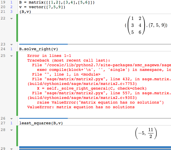
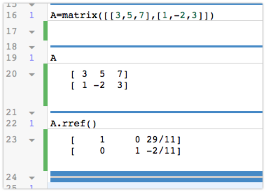
Given a matrix A, A.singular_values() returns the singular values of A, and A.SVD() gives the singular value decomposition. There’s a wrinkle, though: Sage only knows how to compute A.SVD() for certain kinds of matrices, like matrices of floats. So, for instance:
A = matrix([[1,2,3],[4,5,6]])
A.SVD()
gives an error, while
A = matrix(RDF,[[1,2,3],[4,5,6]])
A.SVD()
works fine. (Here, “RDF” stands for “real decimal field”; this tells Sage we want to think of the entries as finite-precision real numbers.)

The command A.SVD() returns a triple (U,S,V) so that A=USV^T; U and V are orthogonal matrices; and S is a “diagonal” (but not square) matrix. So, the columns of U are left singular vectors of A, and the columns of V are right singular vectors of A.

I find the output of A.SVD() hard to read, so I like to look at its three components separately, with:
A.SVD()[0]
A.SVD()[1]
A.SVD()[2]

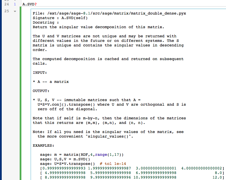
As always, you can get some help by typing
A.svd?

Getting some data

We’ll compute an SVD for some weather data, provided by the National Oceanic and Atmospheric Administration (NOAA). (The main reason I chose this example is that their data is easy to get hold of. Actually, lots of federal government data is accessible. data.gov keeps track of a lot of it, and census.gov has lots of data useful for social sciences.)

To get some data from NOAA, visit the National Climate Data Center at the NOAA, select “I want to search for data at a particular location”, and then select “Search Tool”.  Then hack around for a while until you have some interesting data, and download it. This took me several tries (and each try takes a few minutes):  lots of the monitoring stations were not reporting the data I wanted, but this wasn’t obvious until I downloaded it.  That’s how dealing with real-world data is at the moment; in fact, the NOAA data is much easier to get hold of than most.

You want to download the data as a .csv (comma-separated values) file. Here is the .csv file I used: weatherData.csv. My data is from a monitoring station at Vancouver airport (near Portland), with one entry per day of the year in 2015 (so, 365 entries total), recording the amount of precipitation, maximum temperature, minimum temperature, average wind speed, fastest 2 minute wind speed, and fastest 5 second wind speed.

You can open this csv file with Excel or any other spreadsheet. More important for us, Python (and hence Sage) imports csv files fairly easily.

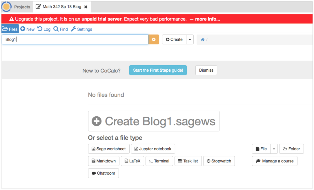
To import the file into Sage, save it to your computer, and then upload it to Sage Math Cloud by clicking “New” (file) button. Here is code that will import the data into a Sage worksheet, once it’s been uploaded to Sage Math Cloud:

import csv
reader=csv.reader(open('weatherData.csv'))
data = []
for row in reader:
     data.append(row)

(If the filename is something other than weatherData.csv, change the first line accordingly.) The result is a list of lists: each line in the data file (spread sheet) is a list of entries, and ‘data’ is a list of those lines. Type

data[0]
data[1]
to get a feeling for what the data looks like.

Converting the data to vectors

We want to:

1. Extract the numerical data from ‘data’, creating a list of vectors (instead of a list of lists).
2. Compute the average of these vectors.
3. Subtract the average from the vectors, creating the “re-centered” or “mean-deviation’ vectors.
4. Turn these re-centered vectors into a matrix A.
5. Compute the singular value decomposition of A.
6. Interpret the result, at least a little.

Step 1. The first real line of data is data[1]. Let’s set
v1=data[1]
v1

The numerical entries of v start at fourth entry, which is v[3] (because Sage counts from 0). To get the part of v starting from entry 3 and going to the end, type
v1[3:]

We want to do this for each line in data, from the second line (line 1) on. We can create a new list of those vectors by:
numerical_vectors = [x[3:] for x in data[1:]]

(As the notation suggests, this creates a list consisting of x[3:] for each line x in data[1:]. This is called list comprehension, (see also Section 3.3 here) and it’s awesome.)

This is still a list of lists. We want to turn it into a list of vectors, in which the entries are real numbers (floating point numbers). A similar command does the trick:
vecs = [vector([float(t) for t in x]) for x in numerical_vectors]

Check that you have what you expect:
data[1]
vecs[0]

Step 2. Computing the average. Note that there are 365 vectors in vecs. (You could ask Sage, which the command len(vecs).)
M = sum(vecs) / 365

Step 3. Again, this is easiest to do using list comprehension:
cvecs = [v - M for v in vecs]

Step 4. This is now easy:
A = matrix(cvecs)

Cleaning the data

The NOAA data is pretty clean — values seem to be pretty reasonable, and in particular of the right type — except that lots of values tend to be missing. Sadly, those missing values get reported as -9999, rather than simply not being present. So, it’s easy to get nonsense computations. For example, if we just type:
A.SVD()[2]

(which gives us the matrix of right singular vectors) something doesn’t look right: many of the entries are very small. Examining our vectors, here’s the problem:
cvecs[19]
data[20]

The last entry here is missing, and reported as -9999.

Dealing with missing data is a hard problem, which is receiving a lot of attention at the moment. We will avoid it just by throwing away the columns that have some missing data. That is, let’s just consider the four columns (precipitation, max temperature, min temperature, average wind speed). I prefer to create new variables with the desired vectors, rather than changing the old ones:
numerical_vectors2 = [x[3:7] for x in data[1:]]
numerical_vectors2[17] #Let's see what one looks like.
vecs2 = [vector([float(t) for t in x]) for x in numerical_vectors2]
M2 = sum(vecs2) / 365
cvecs2 = [v - M2 for v in vecs2]
cvecs2[17] #Let's see what this looks like
A2 = matrix(cvecs2)

SVD and visualizing the result

Now, let’s look at the singular values and vectors.
A2.singular_values()
A2.SVD()[2]

Notice that there’s a pretty big jump between singular values. The third singular value, in particular, is a lot smaller than the first three, so our data should be well approximated by a 3-dimensional space, and even just knowing a 1-dimensional projection of this data should give us a reasonable approximation. Let’s make a list of the singular vectors giving these projections, and look at them a bit more.
sing_vecs = A2.SVD()[2].columns()
sing_vecs[0]

I get roughly (0.0037, -0.8389, -0.5435, -0.0298). This vector stands for (precipitation, maximum temperature, minimum temperature, average windspeed).  This says, for instance, that when the maximum temperature and wind speed also tend to be below average, and the amount of precipitation tends to be above average. (This is consistent with my experience of winter in Oregon, except maybe for the wind speed which is a little surprise.)

The singular vectors give us new coordinates: the new coordinates of a (re-centered) vector are the dot products with the singular vectors:

def coords(v):
     return vector([v.dot_product(w) for w in sing_vecs])

If you look at the coordinates of some of our re-centered vectors, you’ll notice they (almost always) come in decreasing order, and the third is very small. For instance:

coords(cvecs2[17])

(That’s the weather for January 18 that we’re looking at, by the way.)

We can use the coordinates to see how well the data is approximated by 1, 2, and 3-dimensional subspaces. Let’s define functions which give the 1-dimensional, 2-dimensional, and 3-dimensional approximations, and a function that measures the error.

def approx1(v):
     c = coords(v)
     return c[0]*sing_vecs[0]
def approx2(v):
     c = coords(v)
     return c[0]*sing_vecs[0]+c[1]*sing_vecs[1]
def approx3(v):
     c = coords(v)
     return c[0]*sing_vecs[0]+c[1]*sing_vecs[1]+c[2]*sing_vecs[2]
def error(v,w):
     return (v-w).norm()

For example, the approximations for January 18, and the errors are:
v = cvecs2[17]
v
approx1(v)
error(v, approx1(v))
approx2(v)
error(v, approx2(v))
approx3(v)
error(v, approx3(v))

One way to see how good the approximations are is with a scatter plot, showing the sizes of the original vectors and the sizes of the errors between the first, second, and third approximations, for each day in the year:
list_plot([v.norm() for v in cvecs2])+list_plot([error(approx1(v),v) for v in cvecs2], color='red')+list_plot([error(approx2(v),v) for v in cvecs2], color='orange')+list_plot([error(approx3(v),v) for v in cvecs2], color='black')

Blue is the length of the original re-centered data. The red, orange, and black dots are the errors in the first, second, and third approximations. The fact that they get closer to 0, fast, tells you these really are good approximations.

Further thoughts

The data we’ve been looking at is heterogeneous — it doesn’t really make sense to compare the magnitude of the wind speed to the magnitude of the temperature. So, perhaps we should have renormalized all of the components in our vectors first to have standard deviation 1, say, or maybe done something else more complicated. (If we renormalize, we’re blowing up small variations into big ones; is this what we want?) At the very least, our visualization of the errors is a little silly.

Another unsatisfying point is understanding what the second and third singular vectors are telling us, other than that they capture most of the information in the original vectors.

Finally, again, our way of handling missing data is thoroughly unsatisfying. (This is an active area of research, with applications ranging from genomics to music recommendations.)

Least-squares

As far as I know, Sage does not have a built-in method to find a “least-squares solution” to a system of linear equations. The description of a least squares solution to Ax=b as a solution to A^TAx=A^Tb is easy to work with in Sage. For example, to find a least-squares solution to the system

x₁ + x₂ = 3
2x₁ + 3x₂ = 1
x₁ – x₂ = 5

we can type:
A = matrix([[1, 1],[2,3],[1,-1]])
B = A.transpose()
v = vector([3,1,5])
(B*A).solve_right(B*v)

or, more succinctly,
A = matrix([[1, 1],[2,3],[1,-1]])
(A.transpose()*A).solve_right(A.transpose()*vector([3,1,5]))

We could also write a function that finds least-squares solutions for us:

def least_squares(A,v):
     return (A.transpose()*A).solve_right(A.transpose()*v)

(Again, indentation is important: this is Python.) Then we can call it with the matrix and vector of your choice:
B = matrix([[1,2],[3,4],[5,6]])
v = vector([7,5,9])
B.solve_right(v)
least_squares(B,v)

(There is also built-in code in Sage and numpy for fitting curves to data.)

Fourier series

Sage has some rudimentary support for Fourier series, as part of the “piecewise-defined function” class, but it seems to be very slow and very flaky. Let’s implement our own. To make things run reasonably efficiently, we’re going to have Sage do numerical, rather than symbolic, integrals.

As a warm up, to integrate x^2 from 0 to 1, you type:
numerical_integral(x^2,0,1)
The first entry is the answer, while the second is an error estimate.

With this in hand, here’s a function to return a Fourier approximation:

def numerical_fourier(f, n):
    ans = 0
    for i in range(1,n+1):
        ans+= (numerical_integral(f(x)*sin(i*x), -pi,pi)[0])*sin(i*x)/float(pi)
        ans+= (numerical_integral(f(x)*cos(i*x), -pi,pi)[0])*cos(i*x)/float(pi)
    ans+= numerical_integral(f(x),-pi, pi)[0]/(2*float(pi))
    return ans

The inputs to this function are the function you want to approximate, and the number n of sine terms to use.

Let’s approximate the function f(x)=e^sin(x), which is a random-ish periodic function of period 2pi, by a Fourier series with 7 terms:
numerical_fourier(lambda x:exp(sin(x)), 3)


This “lambda x: exp(sin(x))” is a way of quickly defining and passing a function, called lambda calculus.

The answer is not so enlightening. It’s a bit better if we plot it:
plot(exp(sin(x)),(x,-2*pi,2*pi), color='red')
plot(numerical_fourier(lambda x:exp(sin(x)), 3), (x,-2*pi,2*pi))


Let’s plot several Fourier approximations on the same plot, to watch them converging:
plot(exp(sin(x)),(x,-2*pi,2*pi), color="red")+plot(numerical_fourier(lambda x:exp(sin(x)), 1), (x,-2*pi,2*pi), color='green')+plot(numerical_fourier(lambda x:exp(sin(x)), 2), (x,-2*pi,2*pi), color='blue')+plot(numerical_fourier(lambda x:exp(sin(x)), 3), (x,-2*pi,2*pi), color='orange')

It converges pretty quickly — it’s hard to even see the difference between orange (approximation) and red (exact).

These computations are easy in Sage, with some quirks.

Dot products
v=vector([1,2,3])
w = vector([1,1,1])
v.dot_product(w)
v*w
v.norm()

Testing whether sets are orthogonal, orthonormal
The easiest way to test whether a set of vectors v_1, …, v_k is orthogonal is:

1. Create a matrix A=[v_1 … v_k] with the vectors as its columns.
2. Compute A^T*A, the product of the transpose of A with A. The result is diagonal if and only if v_1, …, v_k are orthogonal. The result is the identity if and only if v_1, …, v_k are orthonormal.

This works because the (i,j) entry of A^T*A is the dot product of v_i and v_j.

For example:
v1 = vector([1,1,1,1])
v2 = vector([1,-1,0,0])
v3 = vector([0,0,1,-1])
A = matrix([v1,v2,v3]).transpose()
A
A.transpose()*A


So, these vectors are orthogonal but not orthonormal (which is true–look at them).

v1 = vector([1/2,1/2,1/2,1/2])
v2 = vector([1/sqrt(2),-1/sqrt(2),0,0])
v3 = vector([0,0,1/sqrt(2),-1/sqrt(2)])
A = matrix([v1,v2,v3]).transpose()
A
A.transpose()*A

So, these vectors are orthonormal (again, obviously true).

v1 = vector([1,1,1,1])
v2 = vector([1,1,0,0])
v3 = vector([0,0,1,1])
A = matrix([v1,v2,v3]).transpose()
A
A.transpose()*A

So, these vectors are not orthogonal.

Projections

As far as I know, Sage does not have built in functions for finding orthogonal projects, but writing such functions is fairly easy. This is an optional homework problem.

Gram-Schmidt
Given a matrix A, “A.gram_schmidt(orthonormal=True)” applies the Gram-Schmidt process to the rows of A. The output is a pair of matrices (G,M), so that G is the result of the Gram-Schmidt process and A = M*G. We’re only interested in G in this course.

A second wrinkle is that the Gram-Schmidt process involves taking square roots. If you type a matrix with rational entries, Sage assumes you want to stay in the world of matrices with rational entries. So, for instance,
matrix([[1,2],[3,4]]).gram_schmidt(orthonormal=True)
gives an error.

There seem to be roughly two options to deal with this:

1. Tell Sage you want to work with decimals. The result will be a matrix with ugly decimals, most likely.
2. Tell Sage it’s okay if the resulting matrix has orthogonal but not orthonormal columns (or rather, rows). Then make the rows have length 1 on your own — it’s easy once they’re orthogonal.

For the first option, create your matrix with a command like
A = matrix(RDF,[[1,2],[3,4]])
(RDF stands for “real double field” — the collection of double-precision decimals.) Then
A.gram_schmidt(orthonormal=True)
will behave as expected.

For the second option, just leave off the “orthonormal=True”. For example:
A = matrix([[1,2],[3,4]])
A.gram_schmidt()

Again, note that Sage is applying Gram-Schmidt to the rows. The rows of the first matrix in the output are the result. Notice that they are orthogonal (but not length 1).

Finally, since that was all a bit of a pain, here’s some code which will do Gram-Schmidt to a list of vectors:

def better_gs(vectors):
     A = matrix(vectors)
     G = A.gram_schmidt()[0]
     return [v / v.norm() for v in G.rows()]

(The indentation is important.) If you paste that into your notebook, applying better_gs to a list of vectors should have the result you expect:
v1 = vector([1,2])
v2 = vector([3,4])
better_gs([v1,v2])

This week, the main new computational topic is complex eigenvalues and eigenvectors. Sage finds complex eigenvalues / eigenvectors by default, so we already know how to find complex eigenvectors:
A = matrix([[1,-2],[1,3]])
A.eigenvalues()
A.eigenvectors_right()

Note that Sage uses “I” to stand for i, the square root of -1. (This choice is because “i” is often used as an index, as in “for i=1…5”.) Manipulations work as you would expect:
I^2
z=2+3*I
z
z^2
z+z

Sometimes you want to extract the real part or the imaginary part of a complex number:

z
z.real()
z.imag()

The norm of a complex number a+bi is sqrt(a^2+b^2). Sage (reasonably) calls this the “absolute value”:
z.abs()

The complex conjugate of a+bi is a-bi.
z.conjugate()

We can check some identities, like:
bool(z.abs() == sqrt(z*z.conjugate())
bool(z.real() == (z+z.conjugate())/2)

(The “bool” means we want to know if the expression is true or false, i.e., we want a “boolean“.)

Some things work the same for vectors:
v=vector([1+I,2+3*I])
v.conjugate()
v.real()
Hmm… v.real() didn’t work. We can get around this by using the identity above:

(v+v.conjugate())/2

Another way is to use a bit more Python:
vector([x.real() for x in v])

You can also use exponential (or polar) notation for complex numbers. Use exp(x) for e^x. So:

exp(pi*i)
exp(2*pi*I)
4*exp(pi*I/4)

If we want to convert rectangular representations of complex number to polar ones, we already know how to get the length, with z.abs().  The angle is the argument, so use arg(z). (Why this isn’t z.arg() is a mystery to me.)

arg(z)
arg(i)
arg(1+I)
arg(1+sqrt(3)*I)

As you’ll notice, Sage is remarkably bad at doing this symbolically: it just sort of throws up its hands at 1+sqrt(3)i, where we (of course) know the answer is pi/3. You can always get it to give you a numerical answer, by typing:

float(arg(1+sqrt(3)*I))

We can even torture it into admitting that this is pi/3:

bool(float(arg(1+sqrt(3)*I))==float(pi/3))

Finding eigenvectors and eigenvalues is hard. Our general strategy was:

• Compute the characteristic polynomial. For an n x n matrix, this involves taking the determinant of an n x n matrix with entries polynomials, which is slow. (The fast method for computing determinants, row reduction, doesn’t help much since the entries are polynomials.)
• Find the roots of the characteristic polynomial. You only know a closed form formula for the case n=2. There exist formulas in terms of roots for n=3 and 4, but not for n=5 or higher. You can always approximate the roots using Newton’s method, say, but it’s at best somewhat tedious.
• For each root (eigenvalue), find the corresponding eigenvectors. This involves row reducing a matrix whose entries are perhaps complicated real numbers, once for each eigenvalue.

Fortunately, since finding eigenvalues and eigenvectors is important in practice, there are lots of techniques, and computer code for doing it, symbolically (precisely) and approximately, for general matrices and special classes.

Philosophy over; here are some commands to get started.

Before getting started, to make the output readable, type:
%typeset_mode True

Eigenvalues and eigenvectors in one step.

Let’s create the matrix from Example 5.1.4 in the text, and find its eigenvalues and eigenvectors it:
M = matrix([[4,-1,6],[2,1,6],[2,-1,8]])
M.eigenvectors_right()

Here, Sage gives us a list of triples (eigenvalue, eigenvectors forming a basis for that eigenspace, algebraic multiplicity of the eigenspace). You’re probably most interested in the first two entries at the moment. (As usual, these are column vectors even though Sage displays them as rows.)

We can test these are eigenvectors, by multiplying M by them. For example:
M*vector([1,0,-1/3])
M*vector([1,0,-1/3])==2*vector([1,0,-1/3])

If you just want the list of eigenvalues, type:
M.eigenvalues()


In M.eigenvectors_right(), The word “right” is because we want vectors v so that Mv=cv, not vM=cv. (Why don’t we have to write M.eigenvalues_right()?)

The characteristic polynomial.
M.characteristic_polynomial()

To get the roots of the characteristic polynomial, you can type:
M.characteristic_polynomial().roots()

Sage gives you pairs (root, multiplicity of that root). So, in this case, 2 occurs as a root twice, while 9 occurs once. That is, if we factor the characteristic polynomial we get:

Warning! Sage seems to define the characteristic polynomial to be det(xI – A), while the book and WebWorks use det(A-xI).

Diagonalizing
Not every matrix is diagonalizable, but every matrix has a “Jordan normal form” (which we will not discuss, alas). If the M is diagonalizable then M’s Jordan normal form is diagonal (and conversely). So, to test if M is diagonalizable, you can use:
M.jordan_form()

Alternatively, we can ask for the matrix P so that P^(-1)MP is diagonal. Sage gives this by M. The command is:
M.eigenmatrix_right()

This gives both the matrix P and P^(-1)MP. To extract just P, type:
P = M.eigenmatrix_right()[1]
P


Now we can double check:
P^(-1)*M*P

Sage’s internal help system
If you ever want documentation for a command, just type its name followed by a question mark:
M.eigenmatrix_right?

You can also get a list of possible completions by hitting tab:
M.eigen[TAB KEY]

This post’s goal is to quickly get up to speed with doing linear algebra manipulations in Sage. Work through this, typing the code into Sage. Remember to press shift-return after each piece of code.

Start by creating a new Sage worksheet.

Pretty printing
To make the matrices look nicer, type:
%typeset_mode True
and press shift-return.

Creating matrices
Creating a particular matrix is easy:
matrix([[1,2,3],[4,5,6]])
You can specify the size, though you don’t have to:
matrix(2,3,[[1,2,3],[4,5,6]])

matrix(3,3,[[1,2,3],[4,5,6]])
will generate an error (good); it’s worth getting used to what these look like.

There’s a lot of information in the error message about exactly where the error happened, but the main message is in the last line: “number of rows does not match up with specified number”.

Some particular matrices of interest are the zero matrix and the identity matrix. There’s code to create these:
identity_matrix(3)
zero_matrix(2,3)

(Here, I executed two commands at once, by hitting return after the first but shift-return after the second.)

Often you want to give matrices names:
M = matrix([[1,2,3],[4,5,6]])
I = identity_matrix(3)
This suppresses the output: when you type the above lines and press shift-return, you don’t see any output. To find out the matrices were stored, just type the names and press shift-return:
M
I

Matrix arithmetic
Matrix arithmetic works exactly as you expect, with + for matrix addition, * for matrix multiplication and ^ for matrix exponentiation (when defined); ^ is especially useful for inverses.
M = matrix([[1,2,3],[4,5,6]])
Z = zero_matrix(2,3)
I = identity_matrix(2,2)
N = matrix([[3,1],[4,1]])
N*M
Z+M
M+M
I*M
N^2
N^(-1)
M*M

(The last line should generate an error, of course, and does.)

Vectors
You create vectors with the vector command:
v = vector([1,1,1])
v
You can add vectors, multiply by scalars, and multiply by matrices:
v+v
2*v
M*v

Important. Even though the vectors look like rows, they’re really column vectors.

Row reduction
You row reduce matrices by using the “rref()” function:
M.rref()
matrix([[1,2,3],[0,1,1],[1,3,4]]).rref()

Rank and nullity
Sage computes rank and nullity:
M.rank()
M.right_nullity()

(If you just use M.nullity(), you’ll get the wrong answer: Sage prefers to think of the equation xM=b, not Mx=b, so M.nullity() is the dimension of the space of solutions to xM=0.)

Augmenting matrices
Sometimes it’s convenient to augment a matrix by a vector:
P = matrix([[1,2],[3,4]])
v = vector([-1,-2])
Q=P.augment(v)
P
v
Q

Solving systems of linear equations
Being able to augment and row-reduce is as good as being able to solve Ax=b, but maybe you prefer to have Sage give you the solution directly:
M.solve_right(vector([7,13]))
or
b = vector([7,13])
M.solve_right(b)

Let’s check it’s a solution:
x = M.solve_right(b)
M*x
M*x==vector([7,13])

If you just use M.solve, though, you will get the wrong answer. (Try it!)

Wait a moment… The nullity of M was 1, so there should be a 1-dimensional space of solutions. Sage is not giving the general solution, just one particular solution. (So, augmenting and row-reducing was better.)

What happens if there’s no solution? Try and find out.

And beyond
There’s a lot more we haven’t talked about. (For example, related to last week’s homework, Sage can find bases for null spaces and column spaces for you.) We’ve covered the most useful operations for Math 341; new Math 342 stuff next post.

This post contains detailed instructions for creating your first worksheet on SageMathCloud. It should take you about 15 minutes to work through. (Click on any of the screen shots below for a bigger version.)

1. Visit https://cocalc.com .  You will see a screen where you can create an account:
   
   Click “Create Your Free CoCalc Account!”
   
   Click “I agree to the Terms of Service.” Fill out the form using a real e-mail address and you have an account.
2. You will be taken to a list of your projects (currently blank):
   
   Click “Create New Project”, enter a name (e.g., “Math 342”) and click “Create”.
   
   Then click on the name of your new project.
3. The next step is to create a new file to work in. Type a name (e.g., “Blog1”) and click “Sage worksheet”.
   
4. Your screen should now look like this:
   
   Type “2+2” and press Shift-Return. (That is, hold down the Shift key and press Return.) Sage should compute “4” for you:
   
5. Admittedly, that’s not very impressive. The worksheet has some menus to help you get comfortable with Sage syntax and learn the names of functions. For example, we can graph a function by going to the “Plots” menu select “Function”. You can also plot functions of two variables. Play around with it a bit.
   
6. Sage will (try to) solve systems of equations using the “solve” command. Type:
%var x y
solve([3*x+5*y==7, x-2*y==3],x,y)
   and press shift-return.
   
7. We can also do this using a matrix. To create a matrix, type:
   A=matrix([[3,5,7],[1,-2,3]])
   To get Sage to print your matrix for you, type
   A
   and hit shift-return.
   To get the row-reduced echelon form of A, type:
   A.rref().
   
8. Try entering and row-reducing another matrix, then print out your worksheet and hand it in.  (It’s okay to print it 2 pages per side, to save space.)