Catenary Curves & Vault Workshop Notes (Excerpt)

NOTES IN PROGRESS . FINAL EDIT UNDERWAY

This example is completed in three parts. In Part I,  we build a catenary curve determined by two points. In Part II, we create a series of catenary curves that runs the  along the length of two planar curves. In Part III,  we generate a vault from the series of catenary curves. In Part III three different method are illustrated (Part III A, Part III B, and Part III C). You can simply skip over Part III A and Part III B. For this example Part III C is the most robust method.

Part I. Single Catenary Curve

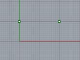
Create two points at arbitrary locations in the plan view in Rhino.

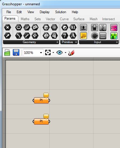
At the command prompt in Rhino type in “Grasshopper” to load the Grasshopper plugin, and from the Parameters (Parmm) tab, place two point symbols in the Canvass window.

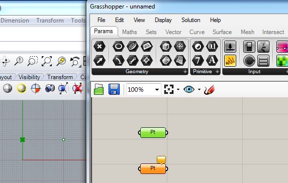
Right-click on  the first “Pt” symbol and choose “set one point” and using the mouse select the  first point  in Rhino (note that you can either select the point directly with the left mouse button, or drag a “rubber banded” selection window around it inside the Rhino view window):

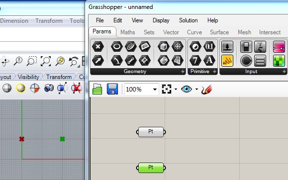
Repeat this so as to connect the second “Pt” symbol with the second of the two points in Rhino.

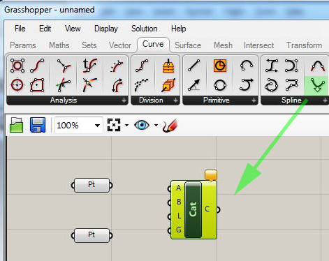
Within “Grasshopper” go to the “Curve” tab, and from the “Spline” area select the “catenary” curve symbol and drag it into the “canvass” window:

  

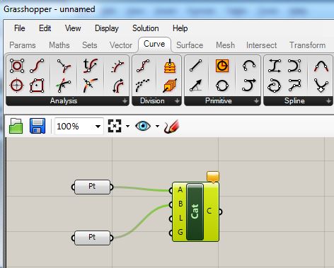
Connect the output port of the first “Pt” to the input port “A” of the “cat” symbol, and connect the output port of the second “Pt” to the input port “B” of the “cat” symbol:

Return to the “Params” tab and drag a numerical input slider into the canvas area:

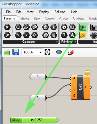
Double-click with the left mouse button directly on the text ” slider”, set its range to be 5  to 150, set its value to 27.5,  and connect its output port to input port “L” of the “cat” symbol.

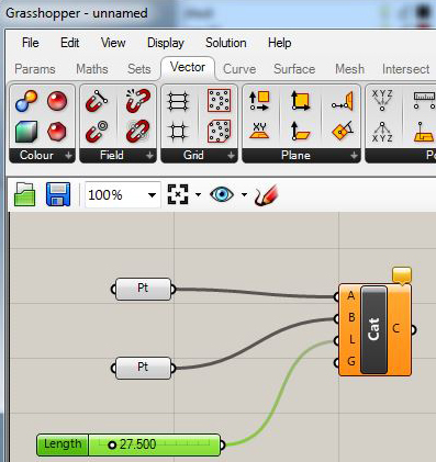
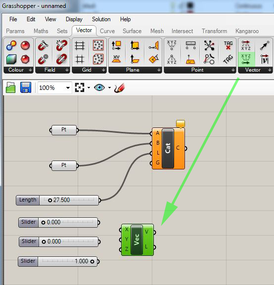
Add three more sliders without modifying their default value ranges.  Next, go to the “Vector” tab, and add a construct vector “symbol” to the canvass.

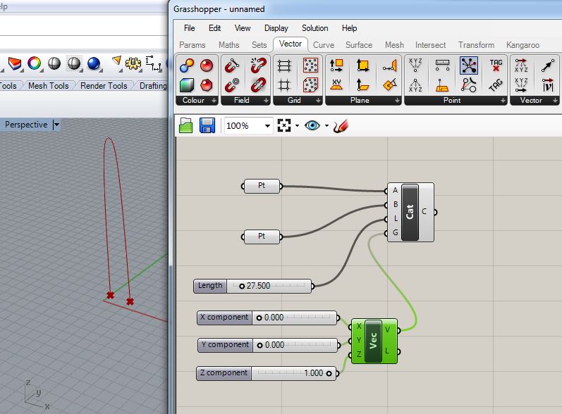
Change the values of the three new sliders to 0.0, 0.0, and 1.0, and connect them to the “X”, “Y” and “Z” input ports of the Vec symbol. Next, connect the “V” output port of the “Vec” symbol to the “G” input port of the “Cat” symbol. Note that a catenary curve is now generated from the two points draping in the negative “Z” direction:

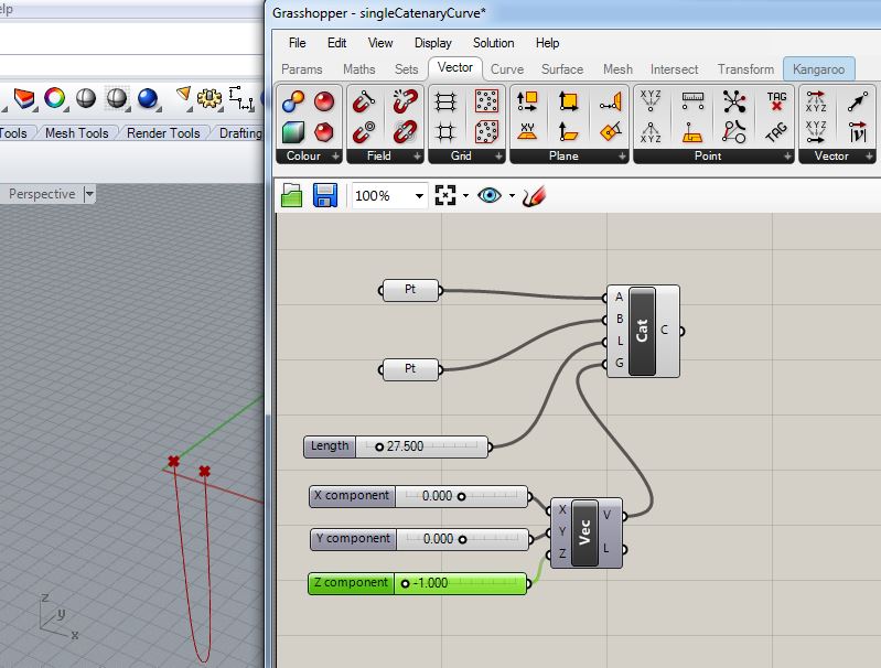
Change the range of each X component, Y component, and Z component sliders to go from -1 to 1. Change their current values to 0.0, 0.0 , and -1.0 respective and note that the catenary curve hands as if pulled in the negative “Z’ axis by gravity.

Part II: Create A Series of Catenary Curves.

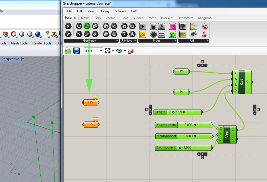
Continuing from Part I, use the  mouse to drag a rectangle  around the current  symbols in the “canvass” window, and then move  them to the right to make way for the two new Grasshopper components. Next, add two simple parallel curves (shown in cyan in the perspective window  below)  in  the Rhino model. Next, in Grasshopper go to the “Params” tab, and drag a “curve” symbol into the “canvass” window.

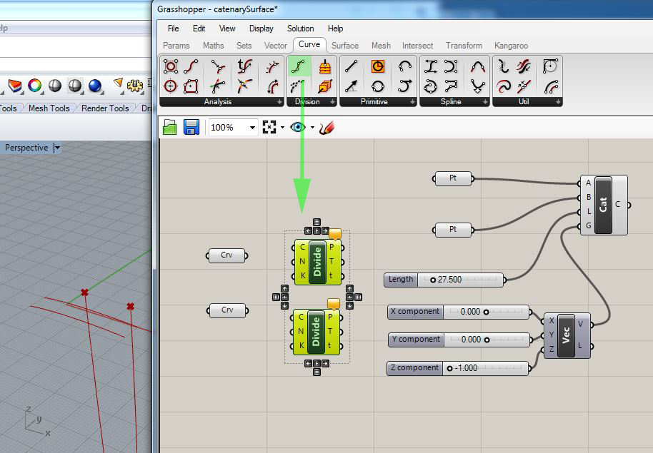
Connect the two new curves in Rhino to the two new “Crv” symbols in the “canvass” window. Now, go to the Grasshopper “Curve” tab, and add two “divide curve” symbols to the “canvass” window:

 

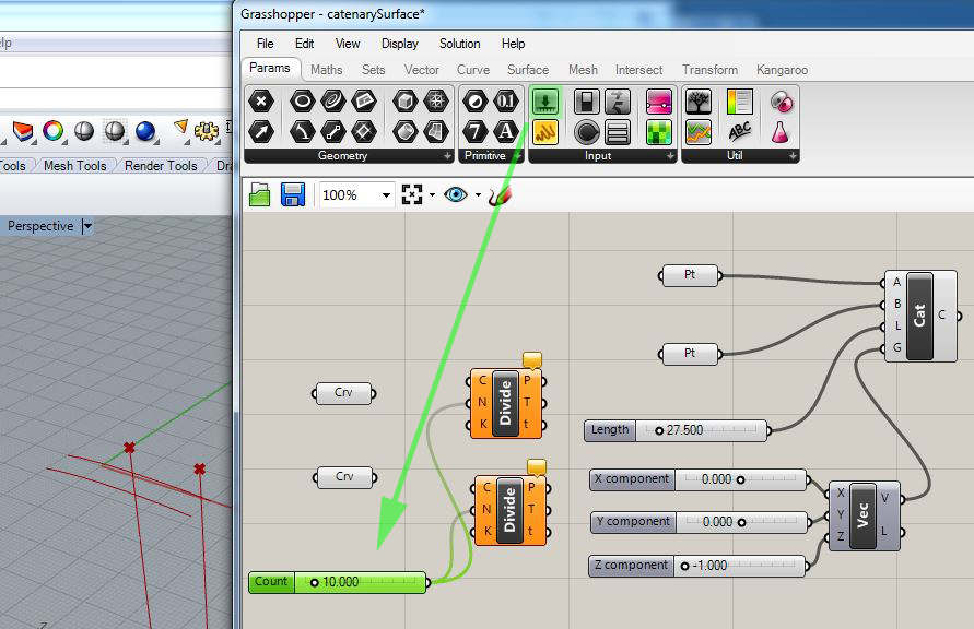
Return to the “Params” tab” and add a new numerical input slider with a range in values of 2 to 100, and set its output port to the “N” input ports of both of the “Divide” symbols.

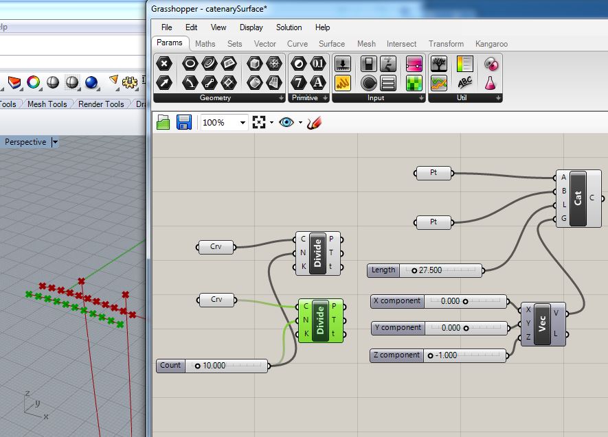
Now, connect the output ports of each of the two “crv” symbols to the corresponding input ports “C” of the “Divide” symbols, and series of points is displayed in Rhino along each of the two new curves.

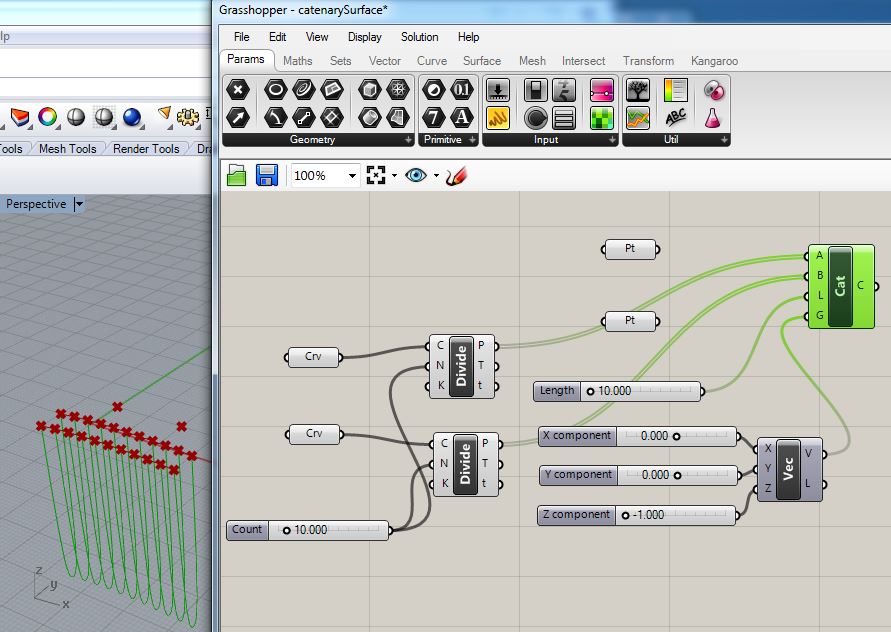
Connect the output ports “P” of the two “Divide” symbols to the corresponding input ports “A” and “B” of the “Cat” symbol. This connection now supplants the connections from the original two points in step 10 above, and a series of Catenary curves is now created. Note too that in this example the “length” slider is reduced from 27.5 to 10.0.

Part III: Create A Vault Surface

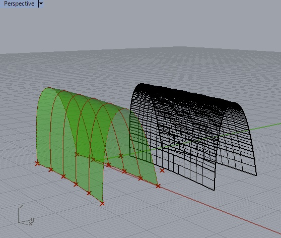
Note that three methods of generating the surface are shown below. The first method uses a “loft” surface. Note that the curves must be relatively simple for this technique to work.There’s a risk that the surface may fold in on itself. If that occurs with the “loft” surface, then try using simpler curves or lessening the “Length” input parameter to the “Cat” symbol. The second method, described further below, uses a “bi-rail” surface which is more likely to result in a coherent surface that isn’t folding in on itself, but still isn’t ideal.  Both methods are shown below. The second method results in the Grasshopper file catenarySurface.ghbased upon the Rhino file makeCatenarySurfaces.3dm (right-click and do a “save as” on these links to download the files). The third option, which is more reliable, relies upon a “network” surface.

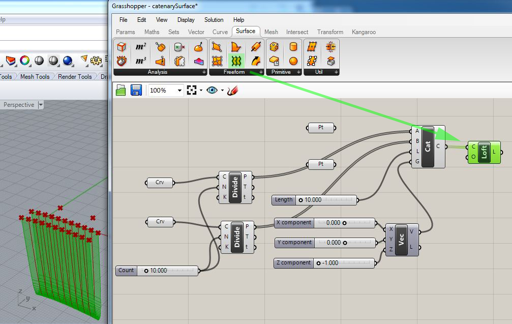
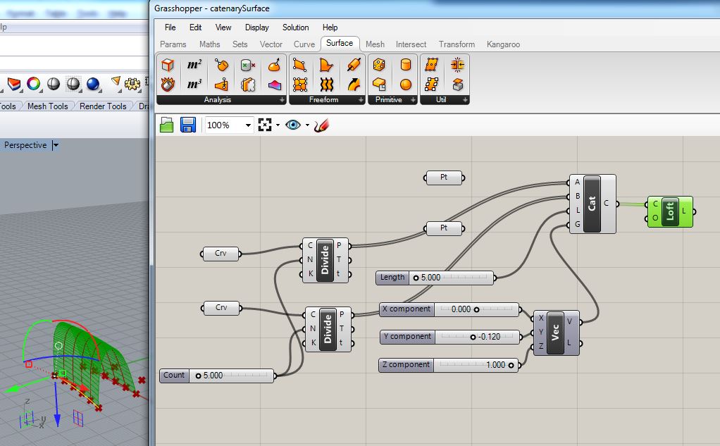
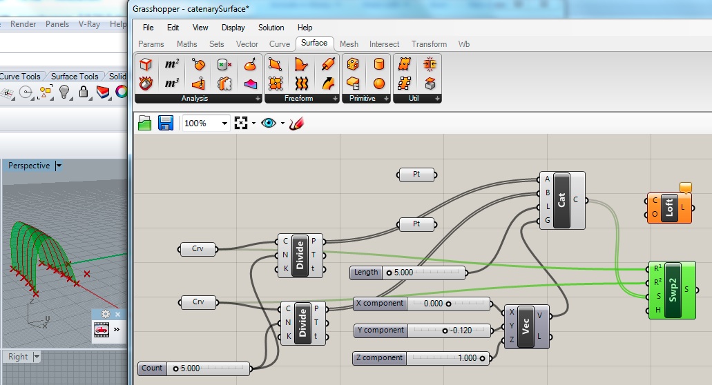
III A. Continuing with the the last example of Part II, go to the “Surface” tab inside of Grasshopper, and add a “loft surface” symbol to the right of the “Cat” symbol. Connect the output port “C” of the “Cat” symbols to the corresponding input port  “C” of the “Loft” symbol. This connection generates a suspended  catenary surface from the two curves.

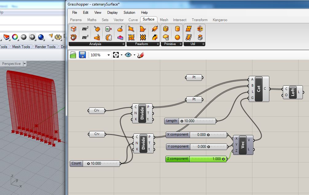
Adjust the value of the “Z component” slider to 1 to have the catenary curve move in the positive “Z” direction.

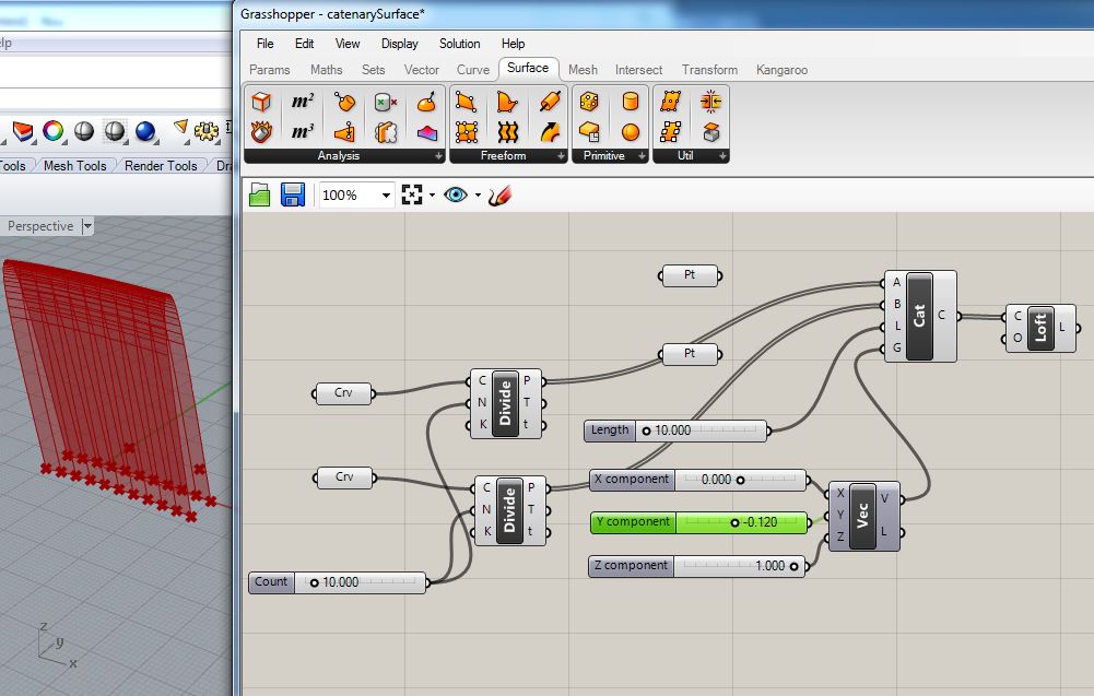
Adjust  the value of the “Y component” slider to -0.12  to cause  the catenary curve to  lean slighty in the negative  “Y” direction.

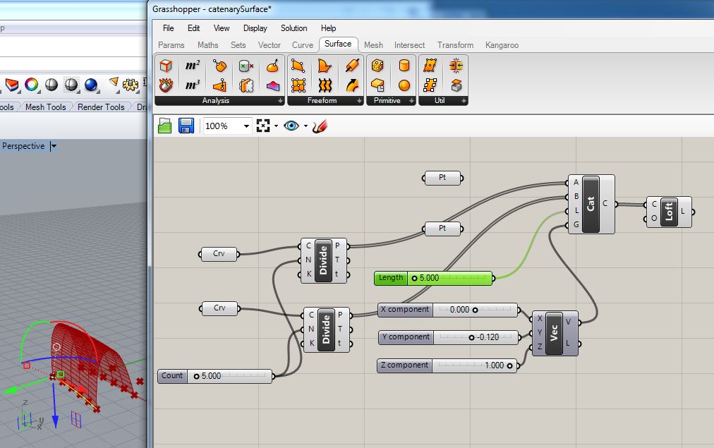
Explore variations in the other numerical sliders, including the “count” slider  to see how the surface is modified. Similary, move or rotate slightly either of the two curves in Rhino and see how the changes in the surface are automatically generated. For example, move the curves in the ground plane further apart, rotate one slighlty, change the number of catenary curves to 5, and the length to 10.

To import the surface more completely inside Rhino, right-clock on the “Loft” symbol  highlighted in green below and from the popup dialog box that follows (not shown below) select the item “Bake”.

III B.  Method 2: BiRail by 2 Rails

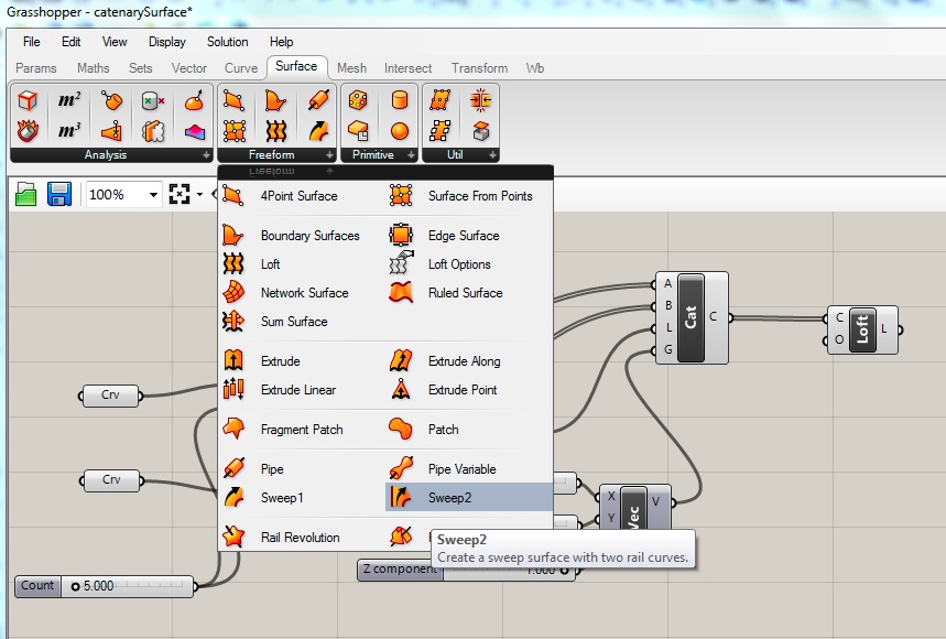
In Grasshopper, to the “Surface” tab, and pulling down the “Freeform” sub-tab, left-click on the “Sweep2” icon and drag it into the canvas window:

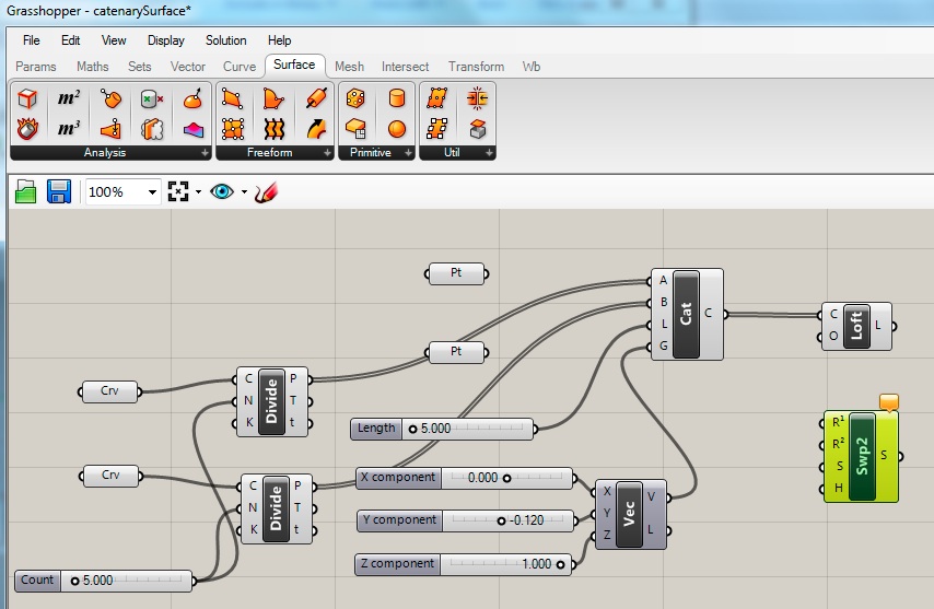
The Birail surface component, shown in green below, has inputs labelled “R1” and “R2” for the two “rail” curves, and “S” for the catenary curve sections:

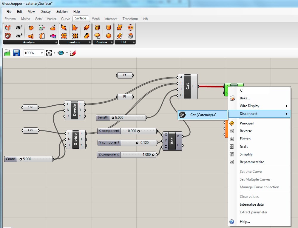
First, within the “canvas” window, right-click on the “loft” component, and select the “disconnect input” option to remove the catenary curves as input.

Next, connect the two “crv” components to “R1 and “R2” and also connect the output port “C” of the “Cat” component to the input port “S” of the “Swp2” component.

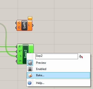
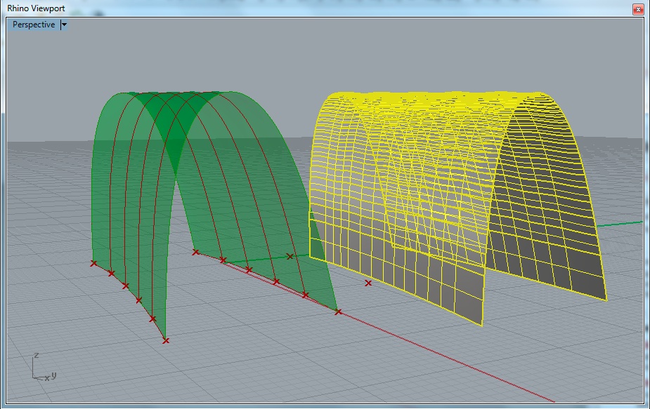
Finally, right-mouse click on the “Swep2” component, and left-mouse click on “Bake” to fully import the surface into Rhino. Once imported, the “baked” surface can be moved and treated like any other polygon surface.

III C. Network surface.

Depending upon the character of the initial curves on the ground, the second method may sometimes also fail. A network surface is yet a third surface type within Grasshopper that tends to be more robust in additional sitautions. The surface is compiled from two sets of curves moving in relatively perpendicular directions along the surface. These are the U and the V directions. Similar to the other two methods, the first step is to go to the “Surface” tab within Grasshopper, and pulling down the “Freeform” sub-tab and left-click on the “Network Surface” icon and drag it into the canvas window:

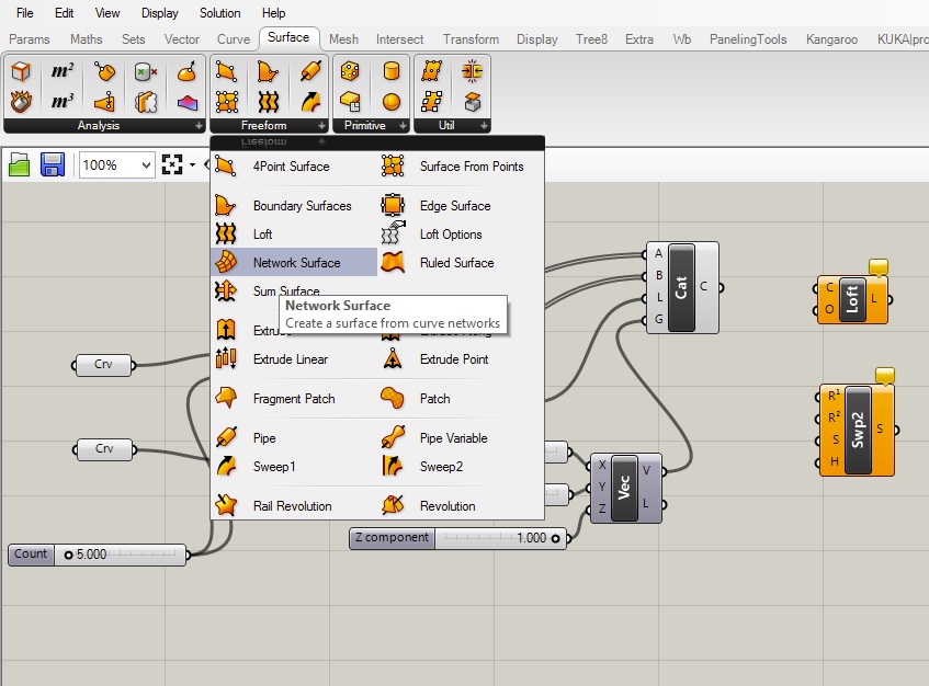
The “Network Surface” component, shown in green below, has inputs labelled “U” and “V” for the two sets of curves. Connect the one of the original “crv” output ports to the “U” input port of the Network Surface. Next, holding down the “shift” key, connect the other one of the “crv” output ports to the “U” input port of the Network Surface. By using the “shift” key, it’s possible to add on the second “crv” to the “U” input port without disconnecting the first one. Next, drag the output port “C” of the catenary curves to the input port “V” of the “Network Surface” component.

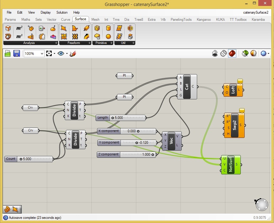
The network surface will now be generated within the Rhino drawing window. Finally, right-mouse click on the “S” output port of the “Network Surface” component, and left-mouse click on “Bake” to fully import the surface into Rhino. Similar to the previous two examples, once imported, the “baked” surface can be moved and treated like any other polygon surface.

This grasshopper file catenarySurface2.gh contains surface components corresponding to the three different methods outlined here. The surface components for the first two surface types have been disconnected from the curve input data, and the component for the third surface type has been connected to this data.