This post’s goal is to quickly get up to speed with doing linear algebra manipulations in Sage. Work through this, typing the code into Sage. Remember to press shift-return after each piece of code.
Start by creating a new Sage worksheet.
Pretty printing
To make the matrices look nicer, type:
%typeset_mode True
and press shift-return.

Creating matrices
Creating a particular matrix is easy:
matrix([[1,2,3],[4,5,6]])
You can specify the size, though you don’t have to:
matrix(2,3,[[1,2,3],[4,5,6]])

matrix(3,3,[[1,2,3],[4,5,6]])
will generate an error (good); it’s worth getting used to what these look like.
There’s a lot of information in the error message about exactly where the error happened, but the main message is in the last line: “number of rows does not match up with specified number”.
Some particular matrices of interest are the zero matrix and the identity matrix. There’s code to create these:
identity_matrix(3)

zero_matrix(2,3)
(Here, I executed two commands at once, by hitting return after the first but shift-return after the second.)
Often you want to give matrices names:
M = matrix([[1,2,3],[4,5,6]])

I = identity_matrix(3)
This suppresses the output: when you type the above lines and press shift-return, you don’t see any output. To find out the matrices were stored, just type the names and press shift-return:
M

I
Matrix arithmetic
Matrix arithmetic works exactly as you expect, with + for matrix addition, * for matrix multiplication and ^ for matrix exponentiation (when defined); ^ is especially useful for inverses.
M = matrix([[1,2,3],[4,5,6]])

Z = zero_matrix(2,3)

I = identity_matrix(2,2)

N = matrix([[3,1],[4,1]])

N*M

Z+M

M+M

I*M

N^2

N^(-1)

M*M
 (The last line should generate an error, of course, and does.)
Vectors
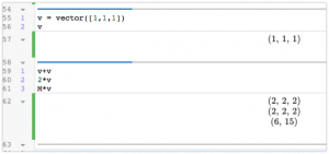
You create vectors with the vector command:
v = vector([1,1,1])

v
You can add vectors, multiply by scalars, and multiply by matrices:
v+v

2*v

M*v
Important. Even though the vectors look like rows, they’re really column vectors.
Row reduction
You row reduce matrices by using the “rref()” function:
M.rref()

matrix([[1,2,3],[0,1,1],[1,3,4]]).rref()
Rank and nullity
Sage computes rank and nullity:
M.rank()

M.right_nullity()
(If you just use M.nullity(), you’ll get the wrong answer: Sage prefers to think of the equation xM=b, not Mx=b, so M.nullity() is the dimension of the space of solutions to xM=0.)
Augmenting matrices
Sometimes it’s convenient to augment a matrix by a vector:
P = matrix([[1,2],[3,4]])

v = vector([-1,-2])

Q=P.augment(v)

P

v

Q
Solving systems of linear equations
Being able to augment and row-reduce is as good as being able to solve Ax=b, but maybe you prefer to have Sage give you the solution directly:
M.solve_right(vector([7,13]))
or
b = vector([7,13])

M.solve_right(b)
Let’s check it’s a solution:
x = M.solve_right(b)

M*x

M*x==vector([7,13])
If you just use M.solve, though, you will get the wrong answer. (Try it!)
Wait a moment… The nullity of M was 1, so there should be a 1-dimensional space of solutions. Sage is not giving the general solution, just one particular solution. (So, augmenting and row-reducing was better.)
What happens if there’s no solution? Try and find out.
And beyond
There’s a lot more we haven’t talked about. (For example, related to last week’s homework, Sage can find bases for null spaces and column spaces for you.) We’ve covered the most useful operations for Math 341; new Math 342 stuff next post.


