Tagged: tutorial

Dealing with “missing”/out of bounds values in heatmaps

I was tinkering around in R to see if I could plot better looking heatmaps, when I encountered an issue regarding how specific values are represented in plots with user-specified restricted ranges. When I’m plotting heatmaps, I usually want to restrict the range of the data being plotted in a specific way. In this case, I was plotting classifier accuracy across frequencies and time of Fourier-transformed EEG data, and I want to restrict the lowest value of the heatmap to be chance level (in this case, 50%).

I used the following code to generate a simple heatmap:

decoding <- readMat("/Users/Pablo/Desktop/testDecoding.mat")$plotData
plotDecoding <- melt(decoding)

quartz(width=5,height=4)
ggplot(plotDecoding, aes(x = Var2, y = Var1)) +
geom_tile(aes(fill = value)) +
scale_fill_viridis(name = "",limits = c(0.5,0.75))

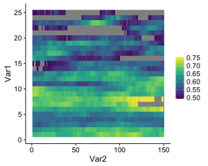
And this is what I got:

heatmap1

See the gray areas? What’s happening here is that any data points that fall outside of my specified data range (see the limits argument in scale_fill_viridis) are being converted to NAs. Apparently, NA values are plotted as gray by default. Obviously these values are not missing in the actual data; how can we actually ensure that they're plotted? The solution comes from the scales package that comes with ggplot. Whenever you create a plot with specified limits, include the argument oob = squish (oob = out of bounds) in the same line where you set the limits (make sure that the scales package is loaded). Ex:

scale_fill_viridis(name = "",limits = c(0.5,0.75),oob=squish)

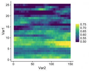
What this does is that values that fall below the specified range are represented as the minimum value (color, in this case), and values that fall above the range are represented as the maximum value (which seems to be what Matlab defaults to). The resulting heatmap looks like this:

heatmap2

A simple solution to an annoying little quirk in R!

611 Highlights in R (Part II)


611 Highlights in R (Part II)


The raw .R file is here and the Rmd file is here.

Brief ‘Hello’ to R Markdown

Let me first introduce you to R markdown and kitr. This format allows you to integrate your analyses with text that can be automatically translated to html, word, and pdf formats. I just produced a supplementary materials document using this and it probably saved me a ridiculous number of hours. It’s easy to get started:

  1. Save your file with extension .Rmd.
  2. Place something like the following in the very top of your file:

    ---
    author: John Flournoy
    title: 611 Highlights in R (Part II)
    output: html_document
    ---
  3. Write as you normally would, using Markdown syntax for formatting. For example:

    # This is a big heading
    
    1. this is
    2. a numbered list
    
    - this is a bulleted list
    - With **bold** and *italic*  text
  4. When you want to throw in some R code, place it inside an R chunk by wrapping it in ```{r} at the beginning and ``` at the end. When you do, it comes out something like this:

    # From Rose's presentation:
    # a toy data set for us to work with
    n <- 100
    gender <- as.factor(c(rep("M", n/2), rep("F", n/2)))
    IQ <- rnorm(n, mean=100, sd=15)
    degree <- rep(c("HS", "BA", "MS", "PhD"), n/4)
    height <- as.numeric(gender)-2 + rnorm(n, mean=5.5, sd=1)
    RT1 <- rchisq(n, 4)
    RT2 <- rchisq(n, 4)
    DV <- 50 - 5*(as.numeric(gender)-1) + .1*IQ + rnorm(n)
    
    df <- data.frame(awesome=DV, gender=gender, IQ=IQ, degree=degree, height=height, RT1=RT1, RT2=RT2)
    head(df)
    ##    awesome gender        IQ degree   height      RT1      RT2
    ## 1 52.89486      M  79.40263     HS 6.292706 1.761990 2.228117
    ## 2 57.04782      M  96.31289     BA 4.759042 2.236027 7.363253
    ## 3 55.59594      M 104.95331     MS 5.560292 5.159114 7.126281
    ## 4 55.44397      M  84.23347    PhD 5.354595 7.652900 2.836956
    ## 5 55.45191      M 107.38754     HS 4.523997 7.768904 4.504664
    ## 6 54.70468      M 110.07096     BA 6.139368 7.786462 7.508488

Notice that in 4, the we see the output of the command head(df). This is useful for outputting tables and plots, as we’ll see.

Here are more resources on

Streamlined Data Workflow with dplyr

Download the data here:

Make sure you have the package (library(dplyr)), and if you don’t, install it (install.packages('dplyr')). Here’s an intro to dplyr straight from the horse’s (Hadley’s) mouth.

By way of data manipulation that I’m actually using for a real project, this tutorial will introduce you to

  • %>%
    • a function chaining operator
  • mutate and transmute
    • adds new variables and preserves existing (transmute drops existing variables)
  • mutate_each
    • adds new variables, applying functions in funs(...) to each column
  • group_by
    • groups data set according to some variable (e.g., gender) – other dplyr operations will be done on groups
  • summarise
    • summarizes multiple values to a single value
  • left_join
    • joins two data frames, returning all rows from x, and all columns from x and y
  • select
    • keeps the variables/columns that you mention (see ?select for special functions that help you select variables)
  • filter
    • returns rows with matching conditions (similar to selecting columns like: aDataFrame[variable == value,])
  • group_by
    • groups data set according to some variable (e.g., gender) – other dplyr operations will be done on groups
  • summarise
    • summarizes multiple values to a single value
  • do
    • use do to perform arbitrary computation, returning either a data frame or arbitrary objects which will be stored in a list (e.g., run the same lm or t.test separately for each gender, country)

Continue reading

simulations

Erik Knight and John Flournoy are working on some simulations to figure out the best way to model cortisol difference scores.

As a general resource for simulation in R, I highly recommend Hadley Wickham’s simulation presntation. Also, the psych package has some great tools for generating data (with great support in this helpful guide by William Revelle).

You can download the code for our example as an Rmd, or as straight R (with R-notebook style comments). You can also walk through the compiled Rmd.

centering and standardizing with scale()

Welcome to some handy functions! These are quick ways to get some common tasks done: centering, standardizing, and getting stats (i.e. mean) for each level of a factor.


# get some data to play with
data()
# Ooo! Chickens. Let's use the ChickWeight dataset.
df <- ChickWeight str(df) summary(df) head(df) # ------------------- # # centering # # ------------------- # ?scale df$weight.c <- scale(df$weight, center=TRUE, scale=FALSE) hist(df$weight.c) # ---------------------------- # # scaling (z scores) # # ---------------------------- # df$weight.z <- scale(df$weight, center=TRUE, scale=TRUE) hist(df$weight.z) # ----------------------------------- # # within levels of a factor # # ----------------------------------- # # lots of great ways to do this, here are two (there are so many more!) # strategy number 1 ?ave df$ave.weight <- ave(df$weight, df$Chick) head(df, n=15) # you don't have to stick with the mean. you can put in any function you like. df$max.weight <- ave(df$weight, df$Chick, FUN=max) # you can center within levels of a factor! df$weight.z.within <- ave(df$weight, df$Chick, FUN=scale) head(df, n=15) # strategy number 2 ?by hist(by(df$weight, df$Chick, FUN=mean), main = "How heavy are those chickens??") # note that this one produces only one mean for each chick: length(unique(df$Chick)) length(by(df$weight, df$Chick, FUN=mean)) nrow(df) # you can put in any function you like hist(by(df$weight, df$Chick, FUN=max), main = "What's the fattest those chickens get??")

Welcome to the wonderful world of R!

Getting started

Slides on R basics (including installation):
www.ats.ucla.edu/stat/r/seminars/intro.htm (you may want to toggle the format using the button in the bottom right)

The way to learn R is by using it, so jump into some practice problems. You can use the “practice with datasets” code copied below, or download swirl and play around with that. Or both!

Learning with Swirl

To install swirl, first install R if you haven’t already (see instructions in the slides above), and open it. In the command line, type
install.packages("swirl")
and hit Enter. You need a working internet connection. Once R has installed the package, you also need to load it. Type
library(swirl)
and hit Enter. Once you do that, swirl will take over and start giving you instructions (and peppy feedback!) to take you though the basics of R. Have fun!

Practice with datasets

This is some code for you to work through to practice using datasets in R.

This coordinates (roughly) with the [Intro to R slides from UCLA](http://www.ats.ucla.edu/stat/r/seminars/intro.htm“>www.ats.ucla.edu/stat/r/seminars/intro.htm).

Download the relevant datasets from dropbox:
https://www.dropbox.com/s/cw5hrw62exn3lvx/rclub1_data1.txt
https://www.dropbox.com/s/zvw58hhel8bu3gh/rclub1_data2.sav

Make a note of where these data files get saved when you download them (your downloads folder, maybe? Or the desktop?). You’ll need to know where they are to be able to access them from R.

Note: this is meant to provide practice moving data in and out of R. suggested functions are provided, but you need to fill in the arguments, etc. For help on how to use the functions, enter ?function.name in the command window (e.g. ?read.table).

To save your work, I recommend copying your code into an R script and working from there. In R Studio, go to File > New File > R Script. In R, go to File > New Document. In either case, this will open up a blank text file. You can copy-paste this code there, and then fill in your answers as work through the problems. Any line of text that begins with # is a comment.

First, check out the file: open the file rclub1_data1.txt in a text editor or excel. you’ll see it’s tab-deliminated. now we want to bring it into R so we can use it. before we tell R which file to open, we need to know what folder R is currently set to look in (working directory). If you’re trying unsucessfully to open a file, the first thing you should check is that your wd is correct.

getwd()
## [1] "/Users/TARDIS/Dropbox/RClub/rclub_code"
# if necessary, change wd so it matches the folder where you've got your data files
setwd("/Users/TARDIS/Dropbox/RClub")

# we want to read in the data file, so first you need to learn about the appropriate function (read.table) so you know how to structure the command. You'll want to do this for each new function you use.
?read.table

# now we can tell R to open the file, and save it as an object called df (short for dataframe). you could name it whatever you want, though. the name of the file ("rclub_data1.txt" must be in quotes, so R knows to look for a string matching that rather than to look for an existing object with that name).
df <- read.table("rclub1_data1.txt", header = T, sep = "\t")

# look at the first part of your dataframe, to eyeball the data.
head(df)
##   gender HowSmartTheyAre HowManyPointsTheyGot DidTheyEatBreakfast
## 1      M              95                    3                   Y
## 2      F              85                    3                   Y
## 3      F             114                    1                   Y
## 4      M             108                    2                   Y
## 5      M              98                    3                   Y
## 6      F              86                    3                   Y
# check the last chunk of the dataset, too, just because you're curious.
tail(df)
##    gender HowSmartTheyAre HowManyPointsTheyGot DidTheyEatBreakfast
## 45      F              87                    5                   N
## 46      M             108                    2                   N
## 47      F              91                    3                   N
## 48      M              95                    4                   N
## 49      F             112                    1                   N
## 50      F             104                    1                   N
# actually, let's look at it in a new window. 
View(df)

# get basic information about your dataframe (dimensions, variable types, etc.)
dim(df)
## [1] 50  4
str(df)
## 'data.frame':    50 obs. of  4 variables:
##  $ gender              : Factor w/ 2 levels "F","M": 2 1 1 2 2 1 2 1 2 1 ...
##  $ HowSmartTheyAre     : int  95 85 114 108 98 86 85 107 100 97 ...
##  $ HowManyPointsTheyGot: int  3 3 1 2 3 3 3 5 2 3 ...
##  $ DidTheyEatBreakfast : Factor w/ 2 levels "N","Y": 2 2 2 2 2 2 2 2 1 1 ...
# what are the variable names (column names)?
colnames(df)
## [1] "gender"               "HowSmartTheyAre"      "HowManyPointsTheyGot"
## [4] "DidTheyEatBreakfast"
# you don't like these column names. rename several of the variables.
colnames(df) <- c("gender", "IQ", "Score", "Breakfast?")

# rename just one variable: change "gender" to "male".
colnames(df)[1] <- "male"


# change the coding scheme for "male" from M/F to Y/N. Remeber that "male" is currently a factor variable. Use str() and View() to check how the coding scheme is applied when you change the levels of the variable.
levels(df$male) # check what they are originally first
## [1] "F" "M"
levels(df$male) <- c("N","Y") # change them to what you want

# you notice a typo (the first subject should actually be female, not male). damn RAs and their sloppy data entry! edit just that cell.
df$male[1] <- "N"

# save this dataframe in csv format, so you can open it in other software:
# write.csv()

# open that csv file back in R, because you're fickle. (note that you can also just use read.table to read csv files - they're actually the same function, just with different defaults)
# read.csv()

# and now save it again, but this time as tab-deliminated. or try using other deliminators, if you like (e.g spaces).
# write.table()

# open the file rclub1_data2.sav (an SPSS file). first, learn about read.spss:
?read.spss
## No documentation for 'read.spss' in specified packages and libraries:
## you could try '??read.spss'
# if R can't find the function, use two ?'s to conduct a boarder search:
??read.spss

#read.spss is in the package "foreign". do you have the foreign package attached already?
sessionInfo()
## R version 3.0.2 (2013-09-25)
## Platform: x86_64-apple-darwin10.8.0 (64-bit)
## 
## locale:
## [1] en_US.UTF-8/en_US.UTF-8/en_US.UTF-8/C/en_US.UTF-8/en_US.UTF-8
## 
## attached base packages:
## [1] stats     graphics  grDevices utils     datasets  methods   base     
## 
## loaded via a namespace (and not attached):
## [1] digest_0.6.4     evaluate_0.5.5   formatR_0.10     htmltools_0.2.4 
## [5] knitr_1.6        rmarkdown_0.3.10 stringr_0.6.2    tools_3.0.2
# if not, load the foreign library.
library(foreign)

# now try ?read.spss again, then open the fie rclub1_data2.sav
df <- read.spss("rclub1_data2.sav")
## Warning: rclub1_data2.sav: Unrecognized record type 7, subtype 18
## encountered in system file
## re-encoding from latin1
# check out the dataframe to see what variables you have, how many cases you have, etc. You can use the same functions you used before.

# add a new column on the end with average test score by taking the mean of each person's scores for the three tests
df$TestAve <- (df$Test1 + df$Test2 + df$Test3)/3