Just another University of Oregon Sites site

The topic in class this week is abstract vector spaces. Sage does understand abstract vector spaces (and many other abstract algebraic structures) to some extent, but not in a way that is useful at the level of this class. So, here’s a brief discussion of creating matrices for computational practice.

First, for row reduction practice, it’s nice to be able to create a matrix of a given size and rank, with integer entries which aren’t too huge:
random_matrix(ZZ,4,5,algorithm='echelonizable',rank=3, upper_bound=7)
will create a random 4×5 matrix with rank 3, integer entries (that’s the ZZ), and entries no bigger than 7.

Second, for inverting matrices, it’s nice if A has integer entries and the inverse of A does, too. Since det(AB)=det(A)det(B), if the determinant of A is not +/-1 then the entries of A^-1 will not be integers. The converse is also true, remarkably: if |det(A)|=1 then the entries of A^-1 will be integers. (This is one of the very few useful applications of Cramer’s rule.) So, we need a way of creating matrices with determinant 1 (or -1). Such matrices are called “unimodular”:
random_matrix(ZZ,5,algorithm='unimodular',upper_bound=9)
will create a 5×5 matrix with integer entries, determinant 1, and entries no bigger than 9 (or maybe 8) in absolute value.

Have fun…

Determinants in Sage work exactly how you would expect:
M = matrix([[1,2,3],[4,5,6],[3,2,1]])
M.determinant()

(If you’re surprised you got 0, check the RREF: M is, indeed, singular.)

There are two shortcuts for the determinant, giving exactly the same thing:
M.det()
det(M)

Go wild.

Amazingly, Sage knows what a linear subspace is, and can do basic computations with them. (Why is this amazing? This is a fairly abstract concept to implement on a computer. You can reduce most computations involving subspaces to computations about matrices. Usually, I would expect a human would do that reduction, and then ask a computer to do the matrix computation. Being able to offload both parts, rather than just the second, to the computer is nice, though Sage’s implementation of the concept is not terribly robust.)

We’ve been working with null spaces, column spaces, row spaces, and spans. These work how you would expect in Sage, except with a few twists:

• It’s important to specify where the entries of the matrices live, i.e., that they are rational numbers or real numbers. We will work with rational numbers in this post; to work with real numbers, replace “QQ” by “RR” below. (Subspaces work differently over the integers than over the rationals or reals.)
• The null space is also called the kernel, and Sage uses the word kernel.
• Sage defaults to finding the left kernel of a matrix, i.e., vectors v so that vM=0. In class, we always look at the right kernel, so we have to tell Sage we want the right_kernel.
• Getting Sage to create the span of a list of vectors seems to be tricky. Just make those vectors into the columns of a matrix and use the column space instead.

With this in mind, let’s create some subspaces. Let’s start with the column space and row space:
M = matrix(QQ,[[1,2,3],[4,5,6],[5,7,9],[3,6,9]])
M
C = M.column_space()
C
Sage tells you the dimension of the ambient space (4) and the subspace (2).

The output is actually quite different if you turn on typeset_mode:
%typeset_mode True
C

In both cases, Sage is telling you that a basis for the subspace is given by the transposes of (1,0,1,3) and (0,1,1,0). (Sage likes row vectors.) We can get a basis explicitly, as a list of vectors:
C.basis()
C.dimension()

Row space is just the same, but with column_space replaced by row_space:
R = M.row_space()
R
R.basis()

Next, for the null space, remember the points above.
K = M.right_kernel()
K
K.basis()


Let’s check that this vector really is in the kernel (null space). This is a little tricky: the basis() command returned a list of vectors, with one vector fin it. We have to extract the vector from the list:
v = K.basis()[0]
v
M*v

In case that was confusing, here’s another kernel example:
N = matrix(QQ,[[1,2,3,4,5],[6,7,8,9,10]])
K_new = N.right_kernel()
list_of_vectors = K_new.basis()
list_of_vectors

We can pick out the individual elements of list_of_vectors:
list_of_vectors[0]
list_of_vectors[1]
list_of_vectors[2]


Let’s check some of these are, indeed, in the null space:
N * list_of_vectors[0]
N * list_of_vectors[1]

(If you’ve programmed in Python before, you should be able to check that all of the vectors are in the null space in a single line of code…)

Inverting matrices

The first topic we discussed this week is inverting matrices. This works exactly as you would expect:
M = matrix([[1,2,3],[1,1,1],[3,1,4]])
M.inverse()

As a sanity check:
M * M.inverse()
(Note that the .inverse() comes first in the order of operations, as it should. If we didn’t know Python would do this way, we would add parenthesis — M*(M.inverse()).)

You can also invert a matrix by raising it to the -1’st power:
M^(-1)

Of course, if the matrix is not invertible Sage raises and exception (i.e., gives an error):
M = matrix([[1,2],[4,8]])
M.inverse()
N = matrix([[1,2,3],[4,5,6]])
N.inverse()

In fact, if you look at the last line of the error message, it tells you briefly why the matrix was not invertible (“singular” meaning square but not invertible in the first example, not square in the second example).

LU factorizations
Sage also has built in code for computing LU factorizations. As the textbook notes:

• Not every matrix has an LU factorization, unless one allows L to be permuted lower triangular, i.e., unless one allows pivoting.
• Even if you only consider matrices which have LU factorizations, roundoff error causes problems unless you use partial pivoting when computing the factorization.

The Sage LU factorization code has several options, depending on how much pivoting you want to allow. The function that returns an LU factorization of M is M.LU(). To see its options, type “M.LU?” and press shift-return. (There’s a lot of documentation there, so don’t print it all out.) The option that matches class most closely is M.LU(pivot=”nonzero”), which means “only do row swapping when absolutely necessary”.

I find the output of M.LU illegible unless we turn on pretty printing. So, try:
%typeset_mode True
M.LU(pivot='nonzero')


Hmm…why did we get three matrices? The first matrix is a permutation matrix: it says how you need to permute (swap) the rows in the second matrix L so that LU is right. If no pivoting was needed (i.e., there is an honest LU factorization) then the first matrix will be the identity matrix (like here). By contrast, if we try:
N = matrix([[1,2,3],[2,4,7],[1,1,1]])
N.LU(pivot='nonzero')
then the first matrix is not the identity matrix.

Let’s give names to the matrices in the LU factorization:
(P,L,U) = M.LU(pivot='nonzero')
P
L
U

(P stands for permutation, though you could of course use any names you like.) Next, let’s make sure that LU really is the right thing:
L*U
L*U == M


For N, L*U will not be N:
(P2, L2, U2) = N.LU(pivot='nonzero')
(P2, L2, U2)
L2 * U2
L2 * U2 == N
P2 * L2
P2 * L2 * U2
P2 * L2 * U2 == N

It works…

This week, we talked about matrix addition, scalar multiplication, matrix multiplication, and the transpose. These all work pretty much how you would expect in Sage:

Let’s create some matrices to play with:
%typeset_mode True
M = matrix([[1,2],[3,4],[5,6]])
N = matrix([[3,1],[4,1],[5,9]])
P = matrix([[2,7],[1,8]])
I = identity_matrix(3)
Z = zero_matrix(3,2)
R = random_matrix(ZZ, 2, 2)
[M, N, P, I, R]

We’ve played with all of the commands except random_matrix, which produces a pseudo-random matrix of a given size. In that command, the ZZ says we want the entries to be integers: Z stands for Zahlen, German for “numbers”. (The function random_matrix has lots of options; if you want a description, type “random_matrix?” and press return.) The last line is just so we get a printout of the matrices.

Now, we can do some arithmetic:
M + N
M - N
3*M
M + P
M + Z
M * R
I * M
R * M
M * N
Some of those lines gave errors; hopefully you know why.

To get the transpose of M:
M.transpose()

Let’s test some matrix arithmetic rules, using random matrices (like the book suggests in problems 36 – 39 in Section 2.1).

A = random_matrix(ZZ,3,3)
B = random_matrix(ZZ,3,3)
[A, B]
A*B
B*A
A*B == B*A
A*(3*B)
3*(A*B)
A.transpose()*B.transpose()
(A*B).transpose()
B.transpose() * A.transpose()
(A*B).transpose() == A.transpose()*B.transpose()
(A*B).transpose() == B.transpose()*A.transpose()

Here’s a screenshot:

Of course, your answers will look different: you should have different random matrices. Given that, though, was the behavior what you expected? (If not, review the book or come and talk to me—Sage is right.)

One last word of caution: if you’re not sure what order Sage will apply operations, use parentheses. For example, A*B.transpose() and (A*B).transpose() are different: the transpose takes precedence over the multiplication. (Try it and check.)

In class this week, we’ve been discussing linear independence and linear transformations. There’s not really any new computation in this material: all of the computations boil down to row-reducing matrices (to see if a set of vectors is linearly independent), or multiplying matrices by vectors (to compute a “matrix transformation”). So, this post will be brief, and mention some ways to construct some useful matrices in Sage (with a little Python programming thrown in).

The identity and zero matrices, and the zero vector
Two important matrices, which we’ve seen already and will see more of, are the zero matrix (all entries are zero) and the identity matrix (square, with ones down the diagonal). Sage has special code for creating these.

For the 3×5 zero matrix:
zero_matrix(3,5)

For the 5×5 identity matrix:
identity_matrix(5)

For the length 3 zero vector:
zero_vector(3)

Let’s make sure these have the effect we expect on a vector:
v = vector([1,2,3,4,5])
Z = zero_matrix(3,5)
Z*v
I = identity_matrix(5)
I*v
Z*v == zero_vector(3)


In the last case, Sage says “True”, because it is true that Z*v is equal to the length 3 zero vector. Note the difference between assigning a value to a variable, with a single equal sign (Z = zero_matrix(3,5)) and testing whether two objects are equal, with a double equal sign (Z*v == zero_vector(3)). Think of = as an orders, and == as a question.

Tricks for lists
We’ve been creating vectors by writing vector([1,2,3,4,5]); but what is the [1,2,3,4,5] itself? It’s a Python list — that is, a sequence of objects. You can make lists of anything — lists of vectors, lists of matrices, lists of lists. For example, here is a list of three matrices:
my_list = [matrix([[1,2],[3,4]]), identity_matrix(5),zero_matrix(2,2)]
my_list


(I found the output unreadable, so I turned on “typeset mode”.)

In fact, we have already been using lists of lists, when we write matrix([[1,2],[3,4]]). If you’re new to Python and would like to learn more about lists, try for example Section 3.2 of Dive Into Python.

You can do arithmetic with lists, but it is completely different from arithmetic with vectors. For example, try:

first_list = [1,2,3,4]
second_list = [5,6,7,8]
first_vector = vector(first_list)
second_vector = vector(second_list)
first_list + second_list
first_vector + second_vector
3*first_list
3*first_vector


List arithmetic can be very convenient. For example, here’s another way of defining the length 17 zero vector:
vector(17*[0])
vector(17*[0])==zero_vector(17)

Defining a rotation matrix function Sage (or rather, Python) is a programming language, so we can use it to write new functions. functions begin with the word “def”, and return a value using “return”. Here’s a function that takes in a number x and returns x+2:

def add_two(x):
     return x+2

Try it with:
add_two(17)

In Python, indentation is important: the indentation tells Python where the function starts and ends. Use the tab key to indent as needed. Also, notice the colon after add_two(x):

Our add_two function is not very impressive. Here’s a function which returns the matrix for rotation in the plane by an angle theta:


def rotation_matrix(theta):
     return matrix([[cos(theta),-sin(theta)],[sin(theta),cos(theta)]])

Let’s check that our rotation_matrix gives what we expect for some special theta’s:
rotation_matrix(0)
rotation_matrix(pi/3)
rotation_matrix(pi/2)
rotation_matrix(pi)
rotation_matrix(2*pi)
rotation_matrix(pi/2)*vector([1,0])
rotation_matrix(pi/2)*vector([1,1])

Last week, we saw how to create an account, project, and Sage worksheet in CoCalc, and some basic operations inside the Sage worksheet — arithmetic, plotting, solving systems of equations, creating and row-reducing matrices. This week, we will focus on two topics:

• Vector arithmetic, and
• Understanding solution sets of systems of linear equations.

Start by going to the project you created last week, and create a new Sage worksheet, as described in last week’s post.

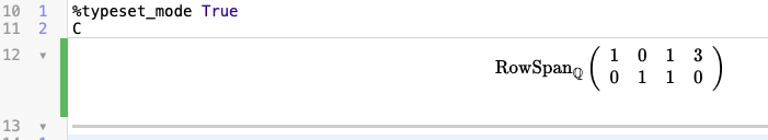
Before we get started, let’s make Sage give us prettier output. Type the following command and press shift-enter:
%typeset_mode True


Vectors
To create a vector named “v” which is equal to the column vector (1,2,3), type:
v=vector([1,2,3])
(Remember to press shift-return.) Typing v by itself and pressing shift-return should show you the vector v:

Even though Sage displays the vector as a row vector, we (and Sage) are going to treat it as a column vector. (As in post 1, click on the screenshot to see a larger version.)

Let’s create a few more vectors and do some vector arithmetic. Type:
w=vector([3,-1,2])
x=vector([1,7])
v+w
3*v
v+x
(Again, remember to press shift-return after each line.)

The output you get should look like this:

In particular, it doesn’t make sense to add v and x, since they have different numbers of entries, and Sage will tell you this with a (somewhat cryptic) error.

All well and good. Sage can also multiply a matrix by a vector:
M = matrix([[1,0,-1],[3,5,3]])
M
M*v
M*w
M*x
The second line is just to get Sage to print out M for you. The product M*x gives an error, as it should: you can’t multiply a 2×3 matrix by a length 2 vector. Your output should look like this:

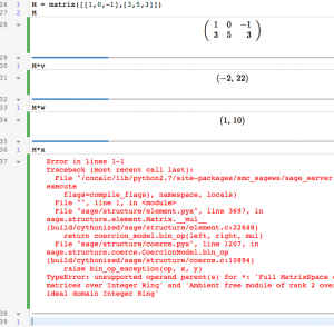
Check the product M*v by hand, to convince yourself Sage got the product right.

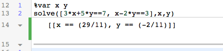
Even better, Sage can solve the matrix equation Mx=b for you, with the command “solve_right”. For example, let’s solve problem 11 in the current edition of Lay-Lay-McDonald’s Linear Algebra:
N = matrix([[1,2,4],[0,1,5],[-2,-4,-3]])
N
b = vector([-2,2,9])
N.solve_right(b)
(The funny syntax — N.solve_right — is because Python, the language underlying Sage, is object-oriented.) Here’s the answer you should get:

Again, even though the answer is displayed as a row vector, read it as a column vector. Check by hand that Nx=b.

Of course, we could do that ourselves by row-reducing. Let’s use Sage to row-reduce the augmented matrix [N|b]:
Nbarb = matrix([[1,2,4,-2],[0,1,5,2],[-2,-4,-3,9]])
Nbarb
Nbarb.rref()

In fact, there’s an even easier way to got an augmented matrix:
N.augment(b)
You can even get straight to the row-reduced form like this:
N.augment(b).rref()

What does solve_right do if there’s no solution? What about if there’s more than one solution? Input an example of each and find out.

Plotting solution sets
There are two ways to describe lines in the plane:

• Implicitly, as the solutions to one equation in two variables. For example, x+2y=3.
• Parametrically, as the set of points swept out as you vary a parameter in the vector equation x=p+tv. For example, (x,y)=(3,0)+t(-2,1).

Sage can plots either. To plot the first kind of equation, use the command:
%var x,y
implicit_plot(x+2*y==3,(x,-5,5),(y,-5,5))

To plot the second kind of equation, use the command:
%var t
p=vector([3,0])
v=vector([-2,1])
parametric_plot(p+t*v,(t,-5,5))

The code we used for the parametric plot is actually needlessly verbose, to get the structure across. Another equivalent version is
%var t
parametric_plot([3-2*t,t],(t,-5,5))

In both cases, the piece (t,-5,5) says we want to see the points where the parameter t runs from -5 to 5. (Since the line is infinite, Sage can’t show the whole line, of course.) In the implicit case, the (x,-5,5) and (y,-5,5) say that the view window should be -5<x

Going back to the implicit plot, recall that varying the number of the right hand side will give parallel lines, with 0 giving a line through the origin. Let’s draw some, in one plot:
implicit_plot(x+2*y==3,(x,-5,5),(y,-5,5))+implicit_plot(x+2*y==0,(x,-5,5),(y,-5,5))+implicit_plot(x+2*y==-2,(x,-5,5),(y,-5,5))+implicit_plot(x+2*y==-1,(x,-5,5),(y,-5,5))
(That’s right — Sage knows how to add plots.)

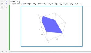
For planes in 3 dimensions, the commands are similar but with “3d” at the end. To plot the plane x+2y+3z=4 use:
%var x y z
implicit_plot3d(x+2*y+3*z==4, (x,-5,5),(y,-5,5),(z,-5,5))

This plane is the same as the parametric plane (x,y,z)=(4,0,0)+s(-3,0,1)+t(0,-3/2,1), which we can plot with:
%var s t
v = vector([-3,0,1])
w = vector([0,-3/2,1])
p = vector([4,0,0])
parametric_plot3d(p+s*v+t*w,(s,-2,2),(t,-2,2))

Finally, let’s loop back to the matrix algebra. If we let M be the 1×3 matrix [1,2,3] then we’ve been looking at the equation Mx=[4]. The vectors v and w in the parametric form should be solutions to the equation Mx=[0], and p should satisfy Mp=4. Let’s check:
M = matrix([1,2,3])
M*v
M*w
M*p

That’s it for today, but we’ve covered a lot.

Since most real-world linear algebra computations are much too large to do by hand, software is essential for practical applications of the material in Math 341. The main software tools that are used are Matlab, Mathematica, and Maple; various extensions of Python; the statistics programming language R; and various low-level languages like C. In this blog, we will use a particular extension of Python, called Sage or CoCalc, for the kinds of computations we are doing in Math 341.

This post contains detailed instructions for creating your first worksheet on CoCalc. It should take you about 15 minutes to work through. (Click on any of the screen shots below for a bigger version.)

1. Visit https://cocalc.com. You will see a screen where you can create an account:
   Fill out the form, using a real e-mail address, and you have an account.
2. You will be taken to a screen where you see a list of projects (currently empty):
   
   Type in a title for your new project and click “Create Project”:
3. Next, add a new worksheet: click “Create or upload files”: Give it a name (like “Week1”) and choose “SageMath Worksheet”:
4. Now we’re in a Sage worksheet; your screen should look like this: Type “2+2” and press Shift-Return. (That is, hold down the Shift key and press Return.) Sage should compute “4” for you:
5. Okay, not so impressive so far. The worksheet has some menus to help you get started with Sage syntax. Let’s try graphing a function. From the “Plots” menu select “Function”. Then press shift-return. You should see a plot of the function.
   
   Play around with the function, and press shift-return to get a new plot. Sage can also do 3D plotting:
6. Time for some linear algebra. Type:
%var x y
solve([3*x+5*y==7, x-2*y==3],x,y)

   
   The first line tells Sage that x and y will be variable names. The second says to solve the pair of equations 3x+5y=7 and x-2y=3 for x and y. (Note the two equal signs in each case.) I will talk about the syntax a little more in a future post.
7. Try solving a few of your homework problems (or other textbook problems) with Sage, to check your work.
8. Finally, let’s create and row-reduce a matrix. To create a matrix, type:
M = matrix([[-3,-8,-22],[1,3,9]])
   (This is one of the matrices from the WebWork homework.) Notice that the syntax is very similar to WebWork. Also note that here we use a single equal sign.To see M, type:
M
and push shift-return.To row-reduce the matrix, type:
M.rref()
   
9. That’s it for the first week. Print out your worksheet (using the printer icon) and hand it in to me, with your name, for a few bonus points.