

This post is part of a series on future-proofing your work (part 1, part 2). Today’s topic is annotating your work files.
Short version: Write a script to annotate your data files in your preferred data analysis program (SPSS and R are discussed as examples). This will let you save data in an open, future-proofed format, without losing labels and other extra information. Even just adding comments to your data files or writing up and annotating your analysis steps can help you and others in the future to figure out what you were doing. Making a “codebook” can also be a good way to accomplish this.
Annotating your files as insurance for the future…
Our goal today is simple: Make it easier to figure out what you were doing with your data, whether one week from now, or one month, or at any point down the road. Think of it this way: if you were hit by a bus and had to come back to your work much later, or have someone else take over for you, would your project come to a screeching halt? Would anyone even know where your data files are, what they represented, or how they were created? If you’re anxiously compiling a mental list of things that you would need to do for anyone else to even find your files, let alone interpret them, read on. I’m going to share a few tips for making this easier with a small amounts of effort.
In the examples below, I’ll be using .sav files for SPSS, a statistics program that’s widely used in my home discipline, Psychology. Even if you don’t use SPSS, though, the same principles should hold with any analysis program.
Annotating within Statistics Scripts:
Commenting Code
Following my post on open vs. closed formats, you likely know that data stored in open formats stand a better chance of being usable in the future. When you save a file in an open format, though, sometimes certain types of extra information get lost. The data themselves should be fine, but extra features, such as labels and other “metadata” (information about the data, such as who created the data file, when it was last modified, etc.), sometimes don’t get carried over.
We can get around this while at the same time making things more transparent to future investigators. One way to do this is to save the data in an open format, such as .csv, and then to save a second, auxiliary file, along with the data to carry that additional information.
Here’s an example:
![]()
SPSS is a popular data analysis program used in the social sciences and beyond. It also uses a proprietary file format, .sav. Thus, we’ll start here with an SPSS file, and move it into an open format.
SPSS has a data window much like any spreadsheet program. Let’s say that a collaborator has given you some data that look like this:
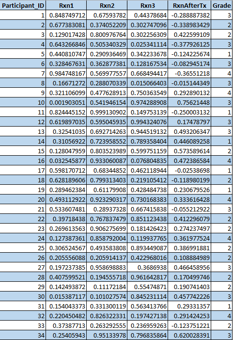
Example Data
Straightforward so far? The data don’t look too complicated: 34 participants (perhaps for a Psychology study), with five variables recorded about each of them. But what does “Rxn1,” the heading of the second variable in the picture, mean? What about “Rxn2?” Does a Grade of “2” mean that the participant is in 2nd grade in school, or that the participant is second-rate in some sport, or something else?
“Ah, but I’ve thought ahead!” your collaborator says smugly. “Look at the ‘Variable’ view in SPSS!” And so we shall:

Example SPSS Variable View
SPSS has a “variable” view that shows metadata about each variable. We can see a better description of what each variable comprises in the “Label” column — “Rxn1,” we can now understand, is a participant’s reaction time on some activity before taking a drug. Your collaborator has even noted in the label for the opaquely-named “RxnAfterTx” variable how that variable was calculated. In addition, if we were to click on the “Values” cell for the “Grade” variable, we would see that 1=Freshman, 2=Sophomore, and so on.
It would have been hard to guess these things from only the short variable names in the dataset. If we want to save the dataset as a .csv file (which is a more open format), one of the drawbacks is that the information from this second screen will be lost. In order to get around that, we can create a new plain-text file that contains commands for SPSS. This file can be saved alongside the .csv data file, and can carry all of that extra metadata information.
In SPSS, comments can be added to scripts in three ways, following this guide (quoted here):
COMMENT This is a comment and will not be executed.
* This is a comment and will continue to be a comment until the terminating period.
/* This is a comment and will continue to be a comment until the terminating asterisk-slash */
We can use comments to add explanations to our new file as we add commands to it. This will actually allows us to add more than the original SPSS file would have held, since we can now have labels as well as the rationale behind them, in the form of comments.
Now able to write comments, we can write and annotate a data-labeling script for SPSS like this:
/* Here you can make notes on your Analysis Plan, perhaps putting the date and your initials to let others know when you last updated things (JL, March 2014): */
/*
Perhaps here you might want to list your analysis goals, so that it’s clear to future readers:
1 Be able to figure out what I was doing.
2 Get interesting results.
*/
/* An explanation of what the code below is doing for anyone reading in the future: Re-label the variables in the dataset so that they match what’s in the example screenshot from earlier in this post: */
VARIABLE LABELS
Participant_ID “” /* The quotes here just mean that Participant_ID has a blank label */
Rxn1 “Reaction time before taking drug”
Rxn2 “Reaction time after first dose of drug”
Rxn3 “Reaction time after second dose of drug”
RxnAfterTx “Rxn1 subtracted from average of Rxn2 and Rxn3”
Grade “Participant’s grade in school”
EXECUTE. /* Tell SPSS to run the command */
/* Now let’s add the value labels to the Grade variable: */
VALUE LABELS
Grade /* For the Grade variable, we’ll define what each value (1, 2, 3, or 4) means. */
1 ‘Freshman’
2 ‘Sophomore’
3 ‘Junior’
4 ‘Senior’
EXECUTE. /* Tell SPSS to run the command. */
Now if we import a .csv version of the data file into SPSS and run the script above, SPSS will have all of the information that the .sav version of the file had.
While this is slightly more work than just saving in .sav format, by saving the data and the accompanying script in plain-text formats, we future-proof them for use by other researchers with other software (although researchers running other software won’t be able to directly run the script above, they will have access to your data and will be able to read through your script, allowing them to understand the steps you took). By saving using plain-text formats, we also make it easier to use more powerful tools, such as version control systems (about which I might write a future post).
By using comments in our scripts (whether they’re accompanying specific data files or not), we enable future readers to understand the rationale behind our analytic decisions. Every programming language can be expected to have a way to make comments. SPSS’ is given above. In R, you just need to add # in front of a comment. In MATLAB, either start a comment with % or use %{ and %} to enclose a block of text that you want to comment out. In whatever language you’re using, the documentation on how to add comments will likely be among the easiest to find.
Other Approaches:
Another, complimentary, approach to making data understandable in the future is to create a “codebook.” A codebook is a document that lists every variable in a dataset, as well as every level (“Freshman,” “Sophomore,” etc.) of each variable, and sometimes provides some summary statistics. It gives a printable summary of what every variable represents.
SPSS can generate codebooks automatically, using the CODEBOOK command. R can do the same, using, for example, the memisc package:
install.packages(‘memisc’)
library(‘memisc’)
?codebook() # Look at the example given in this help file to see how the memisc package allows adding labels to and generating codebooks from R dataframes.
We can also write a codebook manually, perhaps adding it as a block comment to the top of the annotation script. It might start with something like this:
/*
Codebook for this Example Dataset:
Variable Name: Participant_ID
Variable Label (or the wording of the survey question, etc.): Participant ID Number
Variable Name: Rxn1
Variable Label: Reaction time before taking drug
Variable Statistics:
Range: 0.18 to 0.89
Mean: .50
Number of Missing Values: 0
(etc.)*/
Wrapping Up
The use of annotations can save you and your collaborators time in the future by making things clear in the present. In a way, annotating your files (be they data, or code, or summaries of data analysis steps) is a way to accumulate scientific karma. Use these tips to do a favor for future readers, looking forward to a time in the future when you might be treated to the relief of reading over a well-documented file.

